
AI demand forecasting can replace a fixed reorder point with a forecast that reports its own uncertainty, so stock buffers can rise before a peak and fall once it passes. Combined with dynamic safety stock, it turns a number typed into a spreadsheet into a decision recalculated as conditions change.
Many distribution businesses are overstocked and understocked at the same time. The warehouse is full of the wrong things. Cash is tied up in slow movers and seasonal lines that may not shift for months, while the products customers came for have already run out.
That is often less a failure of demand forecasting than a failure of static arithmetic. If a reorder point is fixed in a spreadsheet and revisited once a year, it can be wrong in both directions: too high when demand is quiet and too low when demand spikes.
Here is how the approach works on AWS, and the five design rules worth carrying into any build. Everything below is architecture and approach. It does not describe a verified customer deployment or promise a specific inventory reduction. Results depend on the data, model performance, supplier behavior, business rules and how the forecast is used.
What is AI demand forecasting?
AI demand forecasting uses statistical and machine learning models to estimate how much of each product will sell, by location and period, from sales history and signals such as promotions, prices and holidays. The most useful forecasts return a range, not one number, because the likely error helps determine how much safety stock is needed.
Machine learning demand forecasting differs from basic spreadsheet extrapolation in two practical ways. It can use many signals consistently across a large catalog, and it can learn patterns shared across similar products. The Amazon SageMaker AI DeepAR algorithm, for example, trains on many related time series, accepts features known in advance and returns quantiles of the forecast distribution, according to AWS documentation.
Why a fixed reorder point fails: five problems hiding behind one number
Picture a business distributing fast-moving staples, seasonal lines and long-tail SKUs through regional warehouses. These are three different demand patterns, yet they may be governed by the same blanket logic. Working capital tied up in stock is often a board-level metric, and leadership wants it down without losing sales on the products that move. Underneath the symptom are five distinct problems:
- Cash locked in excess stock. Fixed reorder points and blanket safety buffers can inflate inventory on slow-moving and seasonal SKUs, increasing holding, storage and obsolescence costs.
- Stockouts on high-velocity SKUs. Promotions, festive peaks and regional shifts may not be reflected in reorder levels, so best-sellers can run out before replenishment arrives.
- Forecasts built on history alone. Basic spreadsheet extrapolation often struggles to factor market trends, promotions, pricing and seasonality consistently across a large catalog.
- Supplier variability ignored. Lead times and fill rates differ by supplier, but a common buffer can hide that variation and create either shortages or excess cover.
- Manual, slow replenishment. Reviewing every SKU-location combination by hand can delay purchase orders and introduce errors.
Few of these are purely modeling problems. Most are decision problems that a better forecast only partly solves. That is why the rules below cover the decision as well as the model.
Design rule 1: forecast a range, not a number
The first change is to stop asking the model for a single predicted quantity. A point forecast tells you what demand will probably be, but it does not show how wrong that estimate might be. Safety stock exists to absorb that uncertainty.
Ask the model for a demand range per SKU and location, such as P10, P50 and P90. The P50 is the median estimate. The P10 and P90 mark lower and higher planning values. If the model is well calibrated, actual demand should be at or below the P90 about nine times in ten.
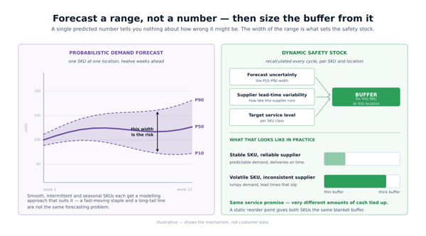
That range is what makes the rest of the system possible. Amazon SageMaker AI Autopilot time-series forecasting uses P10, P50 and P90 by default and lets teams configure the quantiles. AWS also explains quantile forecasting and what-if analysis for retail and consumer packaged goods in its SageMaker Canvas forecasting guide.
Quantiles do not remove judgment. Teams still choose a service level and decide how costly a shortage is relative to excess stock. A high-margin fast mover may justify more protection than a slow or perishable item. Those rules belong in the inventory policy, not inside an unexplained model output.
Design rule 2: segment by demand pattern before choosing an algorithm
Smooth, intermittent and seasonal SKUs behave differently. A fast-moving staple and a long-tail line are not the same forecasting problem and should not automatically be forced through the same model. Segment products by demand pattern, test suitable approaches and retain the one that performs best for the decision horizon. A single approach across the catalog may perform unevenly.
New SKUs with no history can borrow demand patterns from similar products by category, price band and launch season until their own history develops. Models trained across many related series are designed to support this approach, as the DeepAR documentation explains.
Use the signals that explain demand
Sales history is the starting point, not the complete dataset. Add a signal only when it improves backtests or decisions. More columns do not automatically create a better forecast.
| Data group | Examples | Why it matters |
|---|---|---|
| Demand | Orders, units, revenue, returns, cancellations | Defines the target and reveals demand quality |
| Inventory | Stock on hand, open orders, stockouts, transfers | Separates observed sales from constrained demand |
| Commercial | Price, promotions, campaign dates, assortment changes | Explains planned and temporary shifts |
| Calendar | Weekday, month, festivals, holidays, local events | Captures recurring seasonal patterns |
| Supply | Lead time, fill rate, minimum orders, pack sizes | Connects the forecast with replenishment risk |
Two cautions apply. A stockout period is not proof that customers wanted less, so mark it rather than treating it as low demand. A promotion should also be identified so it does not distort the normal baseline.
Design rule 3: size dynamic safety stock from forecast uncertainty and supplier reliability
The width of the forecast range is an important input. Dynamic safety stock is calculated from forecast uncertainty, supplier lead-time variability and the target service level for the SKU class. It is recalculated on a defined schedule rather than entered once and left unchanged.
A stable SKU from a reliable supplier may need a thinner buffer. A volatile SKU from a supplier whose deliveries vary may need a thicker one. Both may carry the same service-level promise while tying up different amounts of cash to keep it.
| Input | What it changes | Control to retain |
|---|---|---|
| Forecast range | Wider uncertainty usually requires a larger buffer | Track calibration and error by SKU segment |
| Supplier lead time | Longer or less reliable delivery increases exposure | Use observed receipts, not contract terms alone |
| Service level | Higher availability targets require more protection | Approve targets by product or customer class |
| Pack size and minimum order | Commercial constraints change the feasible quantity | Validate every recommendation before execution |
| Current stock and open orders | Available and incoming supply reduce the net requirement | Read the authoritative ERP or inventory system |
This is where supplier data earns its place. Lead-time and fill-rate measurements per supplier can directly inform inventory buffers and provide evidence for supplier reviews. For the wider data picture behind these signals, see Rapyder’s guide to supply chain analytics.
How AI demand forecasting fits together on AWS
Sales history from the ERP and point of sale, promotion and price calendars, festive calendars, market signals and supplier delivery records can land in an Amazon S3 data lake. AWS Glue can clean and join them into features keyed by SKU, location and week, while Amazon Athena gives analysts SQL access to the same governed data.
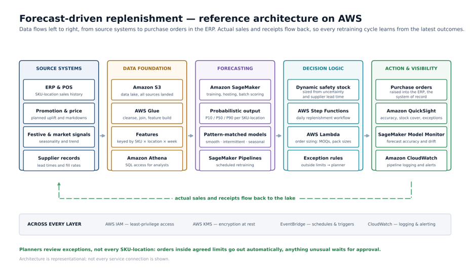
Amazon SageMaker AI can train, evaluate and host the forecasting models. Batch scoring often suits scheduled replenishment, while an API can support interactive planning. SageMaker Pipelines can retrain models on a schedule. Monitoring built on SageMaker AI MLflow Apps and Evidently AI can track forecast accuracy and data drift, while Amazon QuickSight presents accuracy, stock cover and exceptions to planners. AWS IAM controls access, AWS KMS encrypts data at rest and Amazon CloudWatch supports logging and alerts. Actual sales and receipts flow back into the data foundation so each retraining cycle can be evaluated against what happened.
This is a reference design, not a mandatory service list. Match it to data volume, latency needs, team skills and the existing AWS foundation. AWS publishes a current reference in its Guidance for Demand Forecasting for Retail on AWS.
Check service availability before designing the platform. Amazon Forecast has not accepted new customers since 29 July 2024, and AWS directs new use cases toward Amazon SageMaker Canvas. SageMaker Model Monitor closed to new customers effective 30 July 2026. AWS documents open-source SageMaker AI monitoring approaches built on MLflow Apps and Evidently AI, with QuickSight and CloudWatch, as the replacement path.
Design rule 4: automate the routine, escalate the unusual
An exception rule is what makes automated purchasing acceptable to the people accountable for it. It also lets automation expand safely over time.
What happens every day without a planner touching it
A daily AWS Step Functions workflow can compare projected stock against the dynamic reorder point for every SKU and location. Where stock may run short before the next delivery, AWS Lambda can size the order against supplier minimums and pack sizes and submit an approved purchase order to the ERP, which remains the system of record. Anything outside agreed limits waits for a planner.
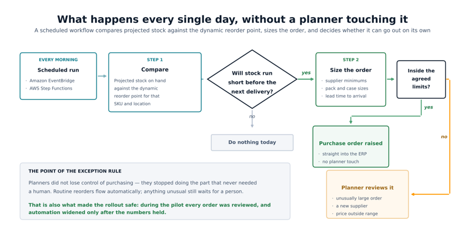
The exception rule is the part worth copying. Planners do not lose control of purchasing. They stop doing the part that does not need a human. Routine reorders inside approved limits can flow automatically. An unusually large order, a new supplier, an unexpected price, stale inventory data or a sharp forecast change still waits for review. Planner attention moves to exceptions, new launches and supplier negotiations.
Because this workflow can write purchase orders, treat it like any automated action: bind approvals to the exact order and protect against duplicates if a call times out.
Design rule 5: gate the rollout on evidence, not on a date
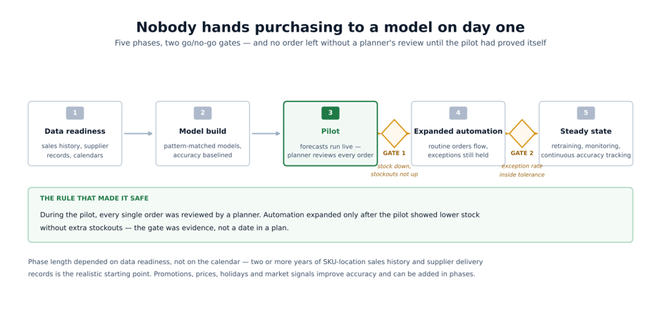
Nobody should hand purchasing to a model on day one. A controlled rollout can move through data readiness, model development, a pilot, expanded automation and steady-state operation. During the pilot, every recommendation should be reviewed. Automation should expand only after the pilot demonstrates lower stock without additional stockouts.
Run the pilot like this:
- Select one category, region or warehouse with enough history and a clear owner.
- Document the current forecast, reorder logic, service target and baseline outcomes.
- Build backtests covering normal periods, promotions, seasonal peaks and stockout periods.
- Run recommendations in parallel with the current process and record planner corrections.
- Automate only cases that meet agreed confidence, business-rule and value limits.
- Review results by SKU segment and decision horizon before expanding scope.
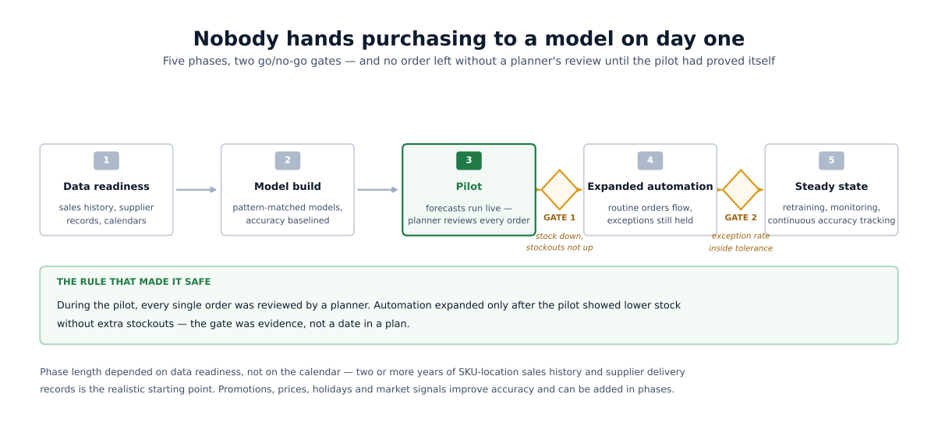
The first gate should require stock to fall without stockouts rising. Before wider automation, the exception rate should also sit within an agreed tolerance. This sequencing takes discipline to plan and makes the result easier to trust.
Phase length depends on data readiness rather than the calendar. Two or more years of SKU-location sales history and supplier delivery records can be a useful starting point, but it is not a universal threshold. Promotions, prices, holidays and market signals can be added in phases rather than treated as prerequisites.
What to measure
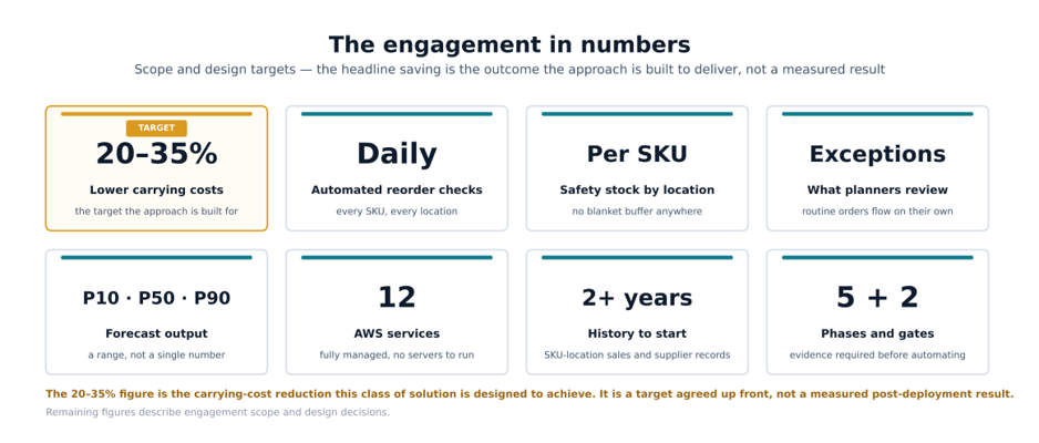
Done well, this class of solution is designed to improve availability on best-sellers as buffers rise before promotions and festive peaks, return planner time to exceptions and supplier negotiations, create per-supplier accountability through lead-time and fill-rate measurement, and establish a data foundation that can support adjacent pricing, assortment and logistics use cases. The principal financial outcome to test is whether carrying cost falls without availability declining.
Forecast accuracy matters, but it is not the final business outcome. Record a baseline before the build, including carrying cost. Track model metrics at the same granularity and horizon used for replenishment, then connect them to availability, inventory and planner effort. A model can improve average error while still failing on the products or periods that matter most.
| Measure | Question it answers |
|---|---|
| Weighted absolute percentage error, or another agreed forecast metric | Is forecast error improving for the demand volume that matters? |
| Quantile coverage | Do actual outcomes fall at or below each stated quantile as often as expected? |
| Stockout rate and fill rate | Did availability improve or decline? |
| Inventory turns and days of cover | Did working capital move without hiding shortages? |
| Exception rate and planner effort | Is automation reducing work or only moving it? |
| Cost per accepted recommendation | Does the benefit justify inference, data and review costs? |
Any savings figure should be a target agreed before the build and tracked against a baseline, not a number implied as already achieved. Published reduction figures depend on the starting inventory policy, so treat them as hypotheses to test.
Where this applies next
Strip out the inventory vocabulary and the pattern is general: quantify uncertainty, size the buffer from it, automate the routine decision, escalate unusual cases and gate the rollout on evidence. The same shape may fit workforce scheduling, capacity planning, cash-flow and collections forecasting, spare-parts provisioning and service-level commitments. The details differ, so test the approach on the organization’s own data first.
Where Rapyder fits
A project like this draws on Rapyder’s AWS machine learning consulting services, MLOps services, data analytics services and data platform engineering for retail and e-commerce businesses. Rapyder’s role is the data, machine learning and cloud layer: data pipelines, model training and deployment, scheduled retraining and monitoring on AWS. Planning policy, including service levels and supplier terms, remains with the business. For an MLOps example from another sector, see the Altigreen MLOps case study.
Still setting reorder points by hand? Start with a scoping conversation. Review sales and supplier data, baseline current carrying cost and stockout rates, and identify where dynamic replenishment may release working capital first. The first deliverable should be a testable baseline and evaluation plan, not an automation commitment.
Ready to improve inventory decisions with AI demand forecasting?
Bring one planning workflow and its current baseline to a practical scoping conversation.
Frequently Asked Questions
Probabilistic demand forecasting predicts a range of likely demand, such as P10, P50 and P90 values, instead of a single number. The width of that range shows how uncertain demand is, which is what safety stock must cover.
A static reorder point remains fixed until someone changes it. Dynamic safety stock is recalculated each cycle from forecast uncertainty, supplier lead-time variability and the target service level, so it can rise before peaks and fall when demand cools.
Basic spreadsheets usually extend past sales and require manual maintenance. Machine learning demand forecasting can combine sales history with promotions, prices and holidays, learn patterns shared across similar products and report forecast uncertainty. It still needs governed data and a controlled decision process.
Start with SKU-location sales history and supplier delivery records. Two years can help reveal annual seasonality, but it is not a fixed rule. Promotions, prices, holidays and market signals can be added in phases.
No. During the pilot, every recommendation should be reviewed. Later, routine orders inside approved limits may flow automatically, while unusually large orders, new suppliers, unexpected prices and stale data continue to require planner approval.
New SKUs can borrow demand patterns from similar products based on category, price band and launch season until their own history develops. Models trained across many related time series are designed to support this cold-start approach.
Yes. In this reference design, purchase orders and stock positions flow through the ERP APIs or file interfaces, so the ERP remains the authoritative system of record. Integration and recovery behavior should be tested before automation expands.
Amazon Forecast has not accepted new customers since 29 July 2024, although existing customers can continue using it. AWS directs new use cases toward Amazon SageMaker Canvas, while custom forecasting models on Amazon SageMaker AI provide another option.